prediction of Heart Disease

Code

suppressPackageStartupMessages({
  library(ggplot2)
  library(cowplot)
  library(randomForest)
  library(tidyverse)
  library(rpart)
  library(rpart.plot)
  library(caret)
  library(Metrics)
})

Data source and Attribute

Data source and Attribute

1. Age (age)

2. Sex (sex)1

3. Chest Pain Type (cp)

4. Resting Blood Pressure (trestbps)

5. Serum Cholesterol (chol)

6. Fasting Blood Sugar \> 120 mg/dl (fbs)

7. Resting Electrocardiographic Results (restecg)

8. Maximum Heart Rate Achieved (thalach)

9. Exercise Induced Angina (exang)

10. ST Depression Induced by Exercise Relative to Rest (oldpeak)

11. Slope of the Peak Exercise ST Segment (slope)

12. Number of Major Vessels Colored by Flourosopy (ca)

13. Thalassemia (thal)

14. Diagnosis of Heart Disease (num) (Predicted Attribute)

Data collection

Code

 url <- "http://archive.ics.uci.edu/ml/machine-learning-databases/heart-disease/processed.cleveland.data"

    data <- read.csv(url, header=FALSE)
    head(data) 

  V1 V2 V3  V4  V5 V6 V7  V8 V9 V10 V11 V12 V13 V14
1 63  1  1 145 233  1  2 150  0 2.3   3 0.0 6.0   0
2 67  1  4 160 286  0  2 108  1 1.5   2 3.0 3.0   2
3 67  1  4 120 229  0  2 129  1 2.6   2 2.0 7.0   1
4 37  1  3 130 250  0  0 187  0 3.5   3 0.0 3.0   0
5 41  0  2 130 204  0  2 172  0 1.4   1 0.0 3.0   0
6 56  1  2 120 236  0  0 178  0 0.8   1 0.0 3.0   0

Data Cleaning and Preprocessing

• Renaming the columns

Code

colnames(data) <- c(
  "age",
  "sex",# 0 = female, 1 = male
  "cp", # chest pain 
          # 1 = typical angina, 
          # 2 = atypical angina, 
          # 3 = non-anginal pain, 
          # 4 = asymptomatic
  "trestbps", # resting blood pressure (in mm Hg)
  "chol", # serum cholestoral in mg/dl
  "fbs",  # fasting blood sugar if less than 120 mg/dl, 1 = TRUE, 0 = FALSE
  "restecg", # resting electrocardiographic results
          # 1 = normal
          # 2 = having ST-T wave abnormality
          # 3 = showing probable or definite left ventricular hypertrophy
  "thalach", # maximum heart rate achieved
  "exang",   # exercise induced angina, 1 = yes, 0 = no
  "oldpeak", # ST depression induced by exercise relative to rest
  "slope", # the slope of the peak exercise ST segment 
          # 1 = upsloping 
          # 2 = flat 
          # 3 = downsloping 
  "ca", # number of major vessels (0-3) colored by fluoroscopy
  "thal", # this is short of thalium heart scan
          # 3 = normal (no cold spots)
          # 6 = fixed defect (cold spots during rest and exercise)
          # 7 = reversible defect (when cold spots only appear during exercise)
  "hd" # (the predicted attribute) - diagnosis of heart disease 
          # 0 if less than or equal to 50% diameter narrowing
          # 1 if greater than 50% diameter narrowing
  )

head(data)

  age sex cp trestbps chol fbs restecg thalach exang oldpeak slope  ca thal hd
1  63   1  1      145  233   1       2     150     0     2.3     3 0.0  6.0  0
2  67   1  4      160  286   0       2     108     1     1.5     2 3.0  3.0  2
3  67   1  4      120  229   0       2     129     1     2.6     2 2.0  7.0  1
4  37   1  3      130  250   0       0     187     0     3.5     3 0.0  3.0  0
5  41   0  2      130  204   0       2     172     0     1.4     1 0.0  3.0  0
6  56   1  2      120  236   0       0     178     0     0.8     1 0.0  3.0  0

Code

str(data)

'data.frame':   303 obs. of  14 variables:
 $ age     : num  63 67 67 37 41 56 62 57 63 53 ...
 $ sex     : num  1 1 1 1 0 1 0 0 1 1 ...
 $ cp      : num  1 4 4 3 2 2 4 4 4 4 ...
 $ trestbps: num  145 160 120 130 130 120 140 120 130 140 ...
 $ chol    : num  233 286 229 250 204 236 268 354 254 203 ...
 $ fbs     : num  1 0 0 0 0 0 0 0 0 1 ...
 $ restecg : num  2 2 2 0 2 0 2 0 2 2 ...
 $ thalach : num  150 108 129 187 172 178 160 163 147 155 ...
 $ exang   : num  0 1 1 0 0 0 0 1 0 1 ...
 $ oldpeak : num  2.3 1.5 2.6 3.5 1.4 0.8 3.6 0.6 1.4 3.1 ...
 $ slope   : num  3 2 2 3 1 1 3 1 2 3 ...
 $ ca      : chr  "0.0" "3.0" "2.0" "0.0" ...
 $ thal    : chr  "6.0" "3.0" "7.0" "3.0" ...
 $ hd      : int  0 2 1 0 0 0 3 0 2 1 ...

• Changing Data types and Structures

Code

# Replace "?"s with NAs
data <- data %>%
  mutate_all(~ifelse(. == "?", NA, .))

# Clean up factors and convert variables
data <- data %>%
  mutate(sex = factor(ifelse(sex == 0, "F", "M")),
         cp = as.factor(cp),
         fbs = as.factor(fbs),
         restecg = as.factor(restecg),
         exang = as.factor(exang),
         slope = as.factor(slope),
         ca = as.factor(as.integer(ca)), # Convert to factor after converting to integer
         thal = as.factor(as.integer(thal)),
         hd = factor(ifelse(hd == 0, "Healthy", "Unhealthy")))

# Print structure of data
data_hd <-na.omit(data) # Data for modeling
glimpse(data_hd)

Rows: 297
Columns: 14
$ age      <dbl> 63, 67, 67, 37, 41, 56, 62, 57, 63, 53, 57, 56, 56, 44, 52, 5…
$ sex      <fct> M, M, M, M, F, M, F, F, M, M, M, F, M, M, M, M, M, M, F, M, M…
$ cp       <fct> 1, 4, 4, 3, 2, 2, 4, 4, 4, 4, 4, 2, 3, 2, 3, 3, 2, 4, 3, 2, 1…
$ trestbps <dbl> 145, 160, 120, 130, 130, 120, 140, 120, 130, 140, 140, 140, 1…
$ chol     <dbl> 233, 286, 229, 250, 204, 236, 268, 354, 254, 203, 192, 294, 2…
$ fbs      <fct> 1, 0, 0, 0, 0, 0, 0, 0, 0, 1, 0, 0, 1, 0, 1, 0, 0, 0, 0, 0, 0…
$ restecg  <fct> 2, 2, 2, 0, 2, 0, 2, 0, 2, 2, 0, 2, 2, 0, 0, 0, 0, 0, 0, 0, 2…
$ thalach  <dbl> 150, 108, 129, 187, 172, 178, 160, 163, 147, 155, 148, 153, 1…
$ exang    <fct> 0, 1, 1, 0, 0, 0, 0, 1, 0, 1, 0, 0, 1, 0, 0, 0, 0, 0, 0, 0, 1…
$ oldpeak  <dbl> 2.3, 1.5, 2.6, 3.5, 1.4, 0.8, 3.6, 0.6, 1.4, 3.1, 0.4, 1.3, 0…
$ slope    <fct> 3, 2, 2, 3, 1, 1, 3, 1, 2, 3, 2, 2, 2, 1, 1, 1, 3, 1, 1, 1, 2…
$ ca       <fct> 0, 3, 2, 0, 0, 0, 2, 0, 1, 0, 0, 0, 1, 0, 0, 0, 0, 0, 0, 0, 0…
$ thal     <fct> 6, 3, 7, 3, 3, 3, 3, 3, 7, 7, 6, 3, 6, 7, 7, 3, 7, 3, 3, 3, 3…
$ hd       <fct> Healthy, Unhealthy, Unhealthy, Healthy, Healthy, Healthy, Unh…

Code

# Count missing values in each column
missing_values <- colSums(is.na(data_hd))

• Decision Tree

Code

# Set seed for reproducibility
set.seed(42)

# Sample the data into training and testing sets
Z <- sample(2, nrow(data_hd), prob = c(0.8, 0.2), replace = TRUE)
hd_train <- data_hd[Z == 1, ]
hd_test <- data_hd[Z == 2, ]

# Train the rpart model
hd_model <- rpart(formula = hd ~ ., data = hd_train, method = "class")
# Visualize the decision tree
rpart.plot(hd_model, yesno = 2, type = 0,extra = 0)

Code

hd_prediction<-predict(object = hd_model,newdata = hd_test,type = "class")

confusionMatrix(data = hd_prediction,reference = hd_test$hd)

Confusion Matrix and Statistics

           Reference
Prediction  Healthy Unhealthy
  Healthy        22         8
  Unhealthy      10        18
                                          
               Accuracy : 0.6897          
                 95% CI : (0.5546, 0.8046)
    No Information Rate : 0.5517          
    P-Value [Acc > NIR] : 0.02259         
                                          
                  Kappa : 0.3771          
                                          
 Mcnemar's Test P-Value : 0.81366         
                                          
            Sensitivity : 0.6875          
            Specificity : 0.6923          
         Pos Pred Value : 0.7333          
         Neg Pred Value : 0.6429          
             Prevalence : 0.5517          
         Detection Rate : 0.3793          
   Detection Prevalence : 0.5172          
      Balanced Accuracy : 0.6899          
                                          
       'Positive' Class : Healthy         
                                          

Code

accuracy(actual = hd_prediction,hd_test$hd)

[1] 0.6896552

Tree splitting criteria based comparison

Code

## Tree splitting criteria based comparison
# Model training based on gini-based splitting criteria
hd_mode11 <- rpart(formula = hd~.,data = hd_train,method = "class",
parms = list(split = "gini"))
# Model training based o] information gain-based splitting criteria
hd_model2 <- rpart(formula = hd~.,
                   data = hd_train,
                   method = "class", 
                   parms = list (split = "information"))

# Generate class predictions on the test data using gini-based splitting criteria
pred1 <- predict(object = hd_mode11,
newdata = hd_test,type = "class")
confusionMatrix(data = pred1,reference = hd_test$hd)

Confusion Matrix and Statistics

           Reference
Prediction  Healthy Unhealthy
  Healthy        22         8
  Unhealthy      10        18
                                          
               Accuracy : 0.6897          
                 95% CI : (0.5546, 0.8046)
    No Information Rate : 0.5517          
    P-Value [Acc > NIR] : 0.02259         
                                          
                  Kappa : 0.3771          
                                          
 Mcnemar's Test P-Value : 0.81366         
                                          
            Sensitivity : 0.6875          
            Specificity : 0.6923          
         Pos Pred Value : 0.7333          
         Neg Pred Value : 0.6429          
             Prevalence : 0.5517          
         Detection Rate : 0.3793          
   Detection Prevalence : 0.5172          
      Balanced Accuracy : 0.6899          
                                          
       'Positive' Class : Healthy         
                                          

Code

accuracy(actual = pred1,hd_test$hd)

[1] 0.6896552

Code

rpart.plot(hd_mode11, yesno = 2, type = 0,extra = 0)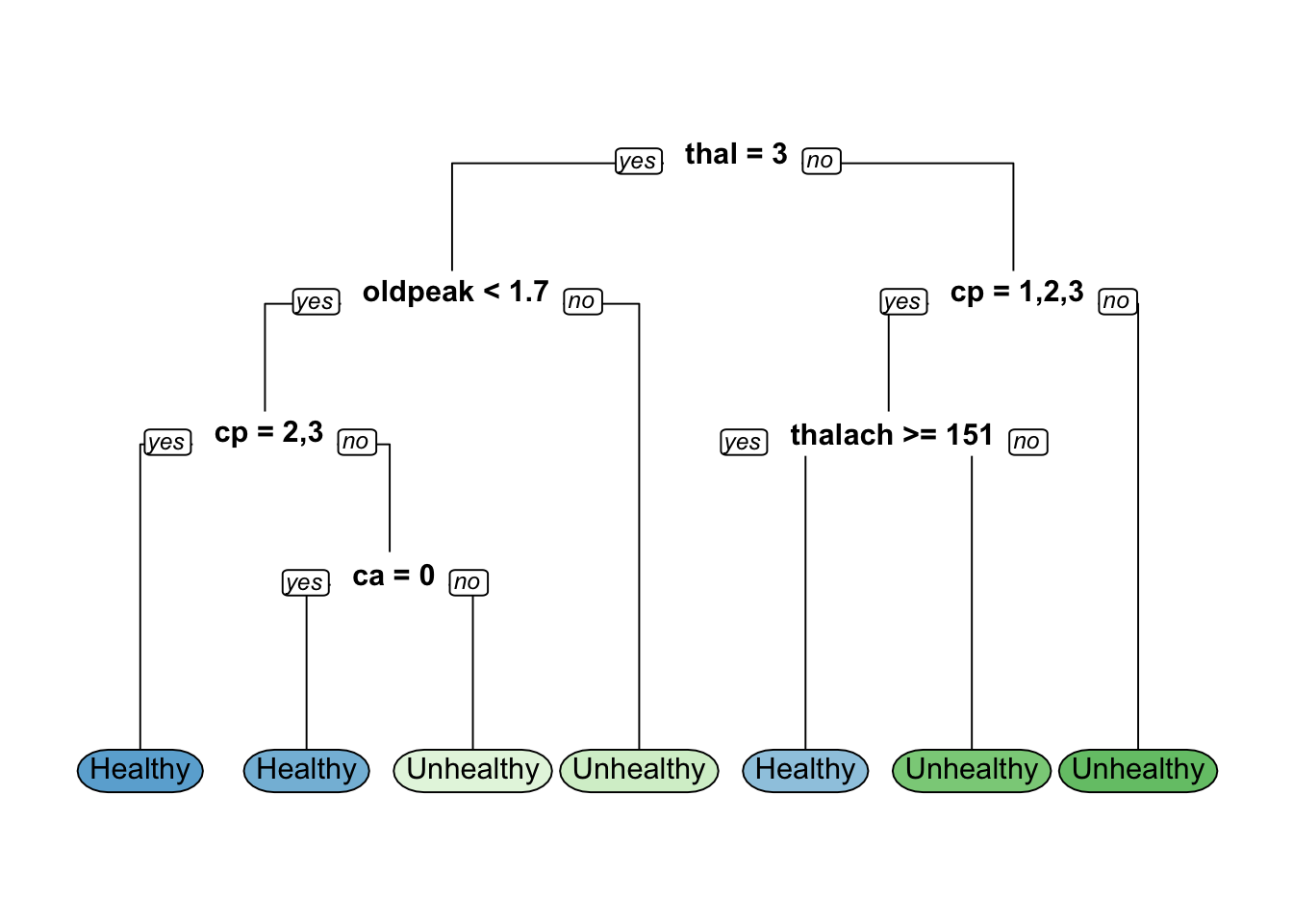

Code

pred2 <- predict(object = hd_model2,
newdata = hd_test,type = "class")

confusionMatrix(data = pred2,reference = hd_test$hd)

Confusion Matrix and Statistics

           Reference
Prediction  Healthy Unhealthy
  Healthy        25         6
  Unhealthy       7        20
                                          
               Accuracy : 0.7759          
                 95% CI : (0.6473, 0.8749)
    No Information Rate : 0.5517          
    P-Value [Acc > NIR] : 0.0003327       
                                          
                  Kappa : 0.5485          
                                          
 Mcnemar's Test P-Value : 1.0000000       
                                          
            Sensitivity : 0.7812          
            Specificity : 0.7692          
         Pos Pred Value : 0.8065          
         Neg Pred Value : 0.7407          
             Prevalence : 0.5517          
         Detection Rate : 0.4310          
   Detection Prevalence : 0.5345          
      Balanced Accuracy : 0.7752          
                                          
       'Positive' Class : Healthy         
                                          

Code

accuracy(actual = pred2,hd_test$hd)

[1] 0.7758621

Code

rpart.plot(hd_model2, yesno = 2, type = 0,extra = 0)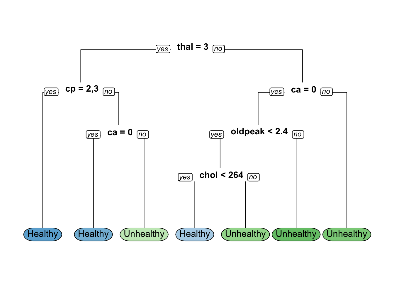

Pruning of Heart model

Code

# Plot the Complexity Parameter (CP) Table
printcp(hd_mode11)

Classification tree:
rpart(formula = hd ~ ., data = hd_train, method = "class", parms = list(split = "gini"))

Variables actually used in tree construction:
[1] ca      cp      oldpeak thal    thalach

Root node error: 111/239 = 0.46444

n= 239 

        CP nsplit rel error  xerror     xstd
1 0.504505      0   1.00000 1.00000 0.069462
2 0.063063      1   0.49550 0.68468 0.064860
3 0.040541      2   0.43243 0.59459 0.062269
4 0.022523      4   0.35135 0.54955 0.060723
5 0.010000      6   0.30631 0.52252 0.059708

Code

# Retrieve the index of the optimal CP value based on cross-validated error
index <- which.min(hd_mode11$cptable[, "xerror"])

# Retrieve the optimal CP value
cp_optimal <- hd_mode11$cptable[index, "CP"]

# Prune the tree based on the optimal CP value
hd_mode11_opt <- prune(tree = hd_mode11, cp = cp_optimal)
hd_mode11_opt

n= 239 

node), split, n, loss, yval, (yprob)
      * denotes terminal node

 1) root 239 111 Healthy (0.53556485 0.46443515)  
   2) thal=3 135  31 Healthy (0.77037037 0.22962963)  
     4) oldpeak< 1.7 120  20 Healthy (0.83333333 0.16666667)  
       8) cp=2,3 76   5 Healthy (0.93421053 0.06578947) *
       9) cp=1,4 44  15 Healthy (0.65909091 0.34090909)  
        18) ca=0 31   6 Healthy (0.80645161 0.19354839) *
        19) ca=1,2 13   4 Unhealthy (0.30769231 0.69230769) *
     5) oldpeak>=1.7 15   4 Unhealthy (0.26666667 0.73333333) *
   3) thal=6,7 104  24 Unhealthy (0.23076923 0.76923077)  
     6) cp=1,2,3 29  14 Healthy (0.51724138 0.48275862)  
      12) thalach>=150.5 15   3 Healthy (0.80000000 0.20000000) *
      13) thalach< 150.5 14   3 Unhealthy (0.21428571 0.78571429) *
     7) cp=4 75   9 Unhealthy (0.12000000 0.88000000) *

Code

## plot optimal model
pred3 <- predict(object = hd_mode11_opt,
newdata = hd_test,type = "class")
confusionMatrix(data = pred1,reference = hd_test$hd)

Confusion Matrix and Statistics

           Reference
Prediction  Healthy Unhealthy
  Healthy        22         8
  Unhealthy      10        18
                                          
               Accuracy : 0.6897          
                 95% CI : (0.5546, 0.8046)
    No Information Rate : 0.5517          
    P-Value [Acc > NIR] : 0.02259         
                                          
                  Kappa : 0.3771          
                                          
 Mcnemar's Test P-Value : 0.81366         
                                          
            Sensitivity : 0.6875          
            Specificity : 0.6923          
         Pos Pred Value : 0.7333          
         Neg Pred Value : 0.6429          
             Prevalence : 0.5517          
         Detection Rate : 0.3793          
   Detection Prevalence : 0.5172          
      Balanced Accuracy : 0.6899          
                                          
       'Positive' Class : Healthy         
                                          

Code

accuracy(actual = pred1,hd_test$hd)

[1] 0.6896552

Code

rpart.plot(hd_mode11_opt, yesno = 2, type = 0,extra = 0)

Hyper parameter Grid Search

Code

## the minimum number of observations that must exist in a node in order for a split 1
## Set the maximum depth of any node of the final tree
minsplit <- seq(1, 20, 1) 
maxdepth <- seq(1, 20, 1)

# Generate a search grid
hyperparam_grid <- expand.grid(minsplit = minsplit, maxdepth = maxdepth)

number_models= nrow(hyperparam_grid)

# create an empty list 

hd_modelling <- list()

## write a loop to save the models
for(i in 1:number_models ){
  minsplit <- hyperparam_grid$minsplit[i]
  maxdepth <- hyperparam_grid$maxdepth[i]
  
  hd_modelling[[i]]<-rpart(formula = hd ~ ., data = hd_train,
                         method = "class",
                         minsplit = minsplit,
                         maxdepth = maxdepth)
  
}


num_models <- length(hd_modelling)
# Create an empty vector to store accuracy values
accuracy_values <- c()
# Use for loop for models accuracy estimation
for (i in 1: num_models) {
# Retrieve the model i from the list
model_heartd <- hd_modelling[[i]]

hd_prediction1<-predict(object = model_heartd,newdata = hd_test,type = "class")

accuracy_values[[i]] <-accuracy(actual = hd_prediction1,hd_test$hd)

}
# Identify the index of the model with maximum accuracy
best_model_index <- which.max(accuracy_values)
# Retrieve the best model
best_model <- hd_modelling[[best_model_index]]
# Print the model hyperparameters of the best model
best_model$control

$minsplit
[1] 1

$minbucket
[1] 0

$cp
[1] 0.01

$maxcompete
[1] 4

$maxsurrogate
[1] 5

$usesurrogate
[1] 2

$surrogatestyle
[1] 0

$maxdepth
[1] 1

$xval
[1] 10

Code

# Calculate accuracy of the best model on test data
pred <- predict(object = best_model, newdata = hd_test, type = "class")
accuracy(actual = hd_test$hd, predicted = pred)

[1] 0.7413793

Code

# Plot the best model
rpart.plot(best_model, yesno = 2, type = 0, extra = 0)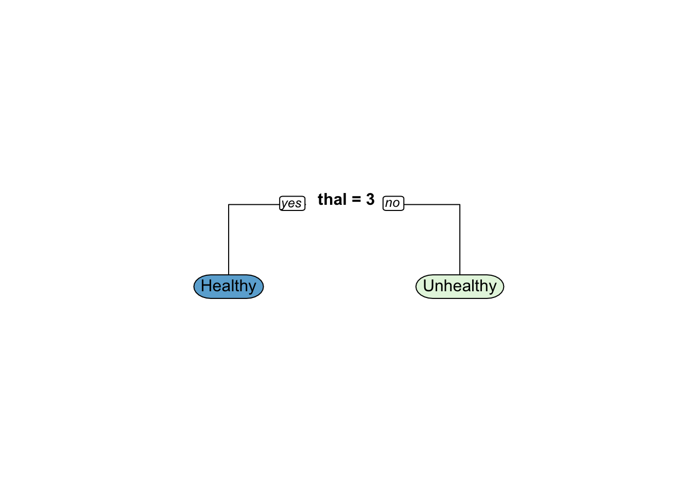

Random forest

• “train” dataset is the bootstrapped data

• “test” dataset is the remaining samples (the “Out-Of-Bag” (OOB) data.)

when we set iter=6, OOB-error bounces around between 17% and 18%. by Breiman

• We want to predict heart disease “hd” with13 variables, and this mtry = sqrt(13) = 3.6 rounded down=3 by default.

Code

set.seed(42)

## impute any missing values in the training set using proximities
data.imputed <- rfImpute(hd ~ ., data = data, iter=6)

ntree      OOB      1      2
  300:  17.49% 12.80% 23.02%
ntree      OOB      1      2
  300:  16.83% 14.02% 20.14%
ntree      OOB      1      2
  300:  17.82% 13.41% 23.02%
ntree      OOB      1      2
  300:  17.49% 14.02% 21.58%
ntree      OOB      1      2
  300:  17.16% 12.80% 22.30%
ntree      OOB      1      2
  300:  18.15% 14.63% 22.30%

Code

model <- randomForest(hd ~ ., data=data.imputed, proximity=TRUE)
model

Call:
 randomForest(formula = hd ~ ., data = data.imputed, proximity = TRUE) 
               Type of random forest: classification
                     Number of trees: 500
No. of variables tried at each split: 3

        OOB estimate of  error rate: 16.83%
Confusion matrix:
          Healthy Unhealthy class.error
Healthy       142        22   0.1341463
Unhealthy      29       110   0.2086331

• Is random forest is actually big enough…

Code

oob.error.data <- data.frame(
  Trees=rep(1:nrow(model$err.rate), times=3),
  Type=rep(c("OOB", "Healthy", "Unhealthy"), each=nrow(model$err.rate)),
  Error=c(model$err.rate[,"OOB"], 
    model$err.rate[,"Healthy"], 
    model$err.rate[,"Unhealthy"]))

ggplot(data=oob.error.data, aes(x=Trees, y=Error)) +
  geom_line(aes(color=Type))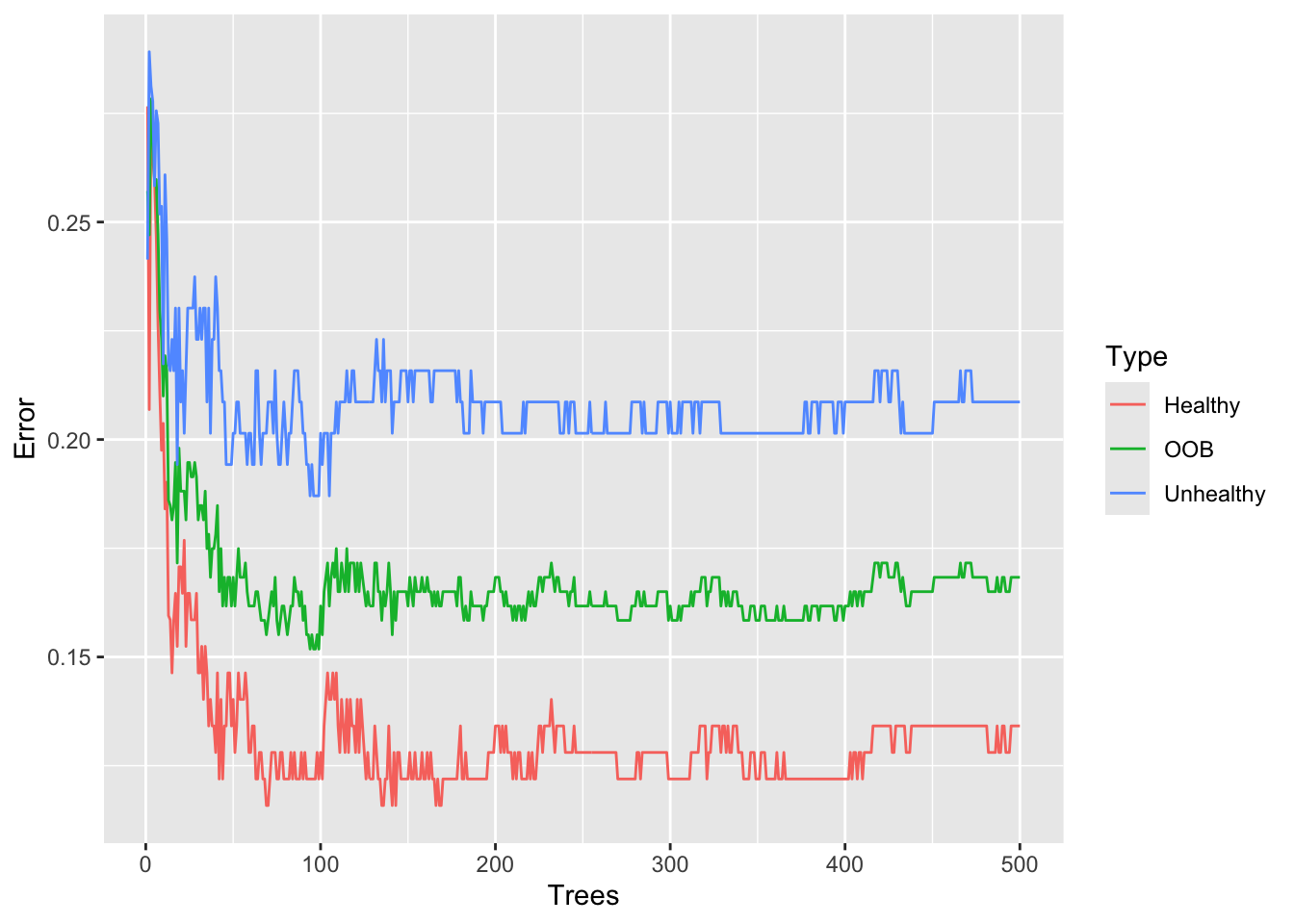

Code

# ggsave("oob_error_rate_500_trees.pdf")

Code

set.seed(42)

model_100 <- randomForest(hd ~ ., data=data.imputed, ntree=1000, proximity=TRUE)
model_100

Call:
 randomForest(formula = hd ~ ., data = data.imputed, ntree = 1000,      proximity = TRUE) 
               Type of random forest: classification
                     Number of trees: 1000
No. of variables tried at each split: 3

        OOB estimate of  error rate: 16.5%
Confusion matrix:
          Healthy Unhealthy class.error
Healthy       144        20   0.1219512
Unhealthy      30       109   0.2158273

Code

oob.error.data <- data.frame(
  Trees=rep(1:nrow(model_100$err.rate), times=3),
  Type=rep(c("OOB", "Healthy", "Unhealthy"), each=nrow(model_100$err.rate)),
  Error=c(model_100$err.rate[,"OOB"], 
    model_100$err.rate[,"Healthy"], 
    model_100$err.rate[,"Unhealthy"]))

ggplot(data=oob.error.data, aes(x=Trees, y=Error)) +
  geom_line(aes(color=Type))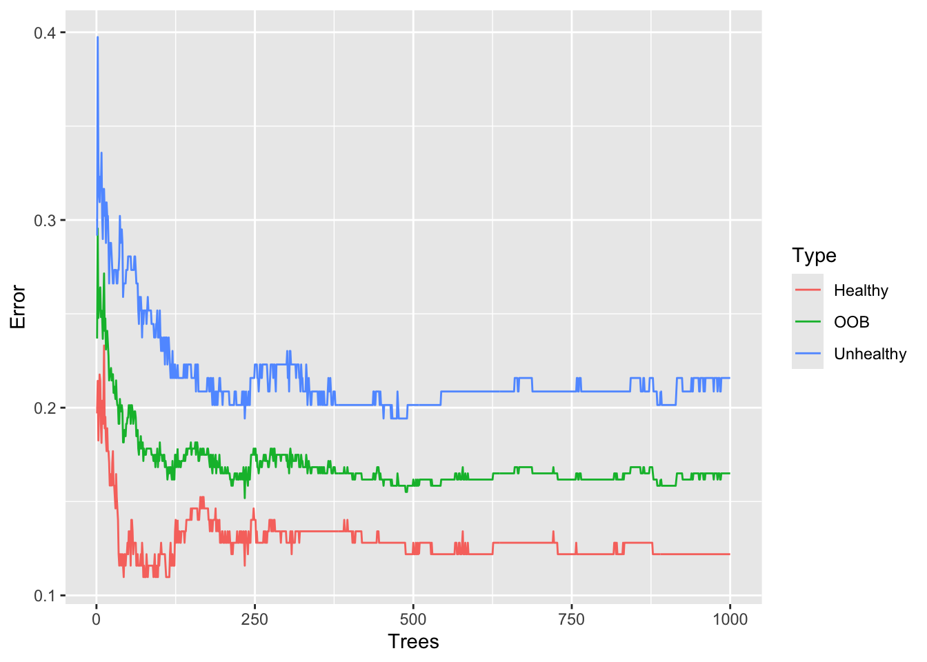

Code

# ggsave("oob_error_rate_1000_trees.pdf")

After building a random forest with 1,000 trees, we get the same OOB-error 16.5% and we can see convergence in the graph. So we could have gotten away with only 500 trees, but we wouldn’t have been sure that number was enough.

• checking if the number of predictors use is optimal

Code

set.seed(42)
## If we want to compare this random forest to others with different values for
## mtry (to control how many variables are considered at each step)...
oob.values <- vector(length=10)
for(i in 1:10) {
  temp.model <- randomForest(hd ~ ., data=data.imputed, mtry=i, ntree=1000)
  oob.values[i] <- temp.model$err.rate[nrow(temp.model$err.rate),1]
}
oob.values

 [1] 0.1749175 0.1749175 0.1716172 0.1815182 0.1815182 0.1815182 0.1782178
 [8] 0.1881188 0.1848185 0.1980198

Code

## find the minimum error
min(oob.values)

[1] 0.1716172

Code

## find the optimal value for mtry...
which(oob.values == min(oob.values))

[1] 3

MDS-plot

Code

set.seed(42)
## create a model for proximities using the best value for mtry
model <- randomForest(hd ~ ., 
                      data=data.imputed,
                      ntree=1000, 
                      proximity=TRUE, 
                      mtry=which(oob.values == min(oob.values)))


## Start by converting the proximity matrix into a distance matrix.
distance.matrix <- as.dist(1-model$proximity)

mds.stuff <- cmdscale(distance.matrix, eig=TRUE, x.ret=TRUE)

## calculate the percentage of variation that each MDS axis accounts for...
mds.var.per <- round(mds.stuff$eig/sum(mds.stuff$eig)*100, 1)

## now make a fancy looking plot that shows the MDS axes and the variation:
mds.values <- mds.stuff$points
mds.data <- data.frame(Sample=rownames(mds.values),
  X=mds.values[,1],
  Y=mds.values[,2],
  Status=data.imputed$hd)

ggplot(data=mds.data, aes(x=X, y=Y, label=Sample)) + 
  geom_text(aes(color=Status)) +
  theme_bw() +
  xlab(paste("MDS1 - ", mds.var.per[1], "%", sep="")) +
  ylab(paste("MDS2 - ", mds.var.per[2], "%", sep="")) +
  ggtitle("MDS plot using (1 - Random Forest Proximities)")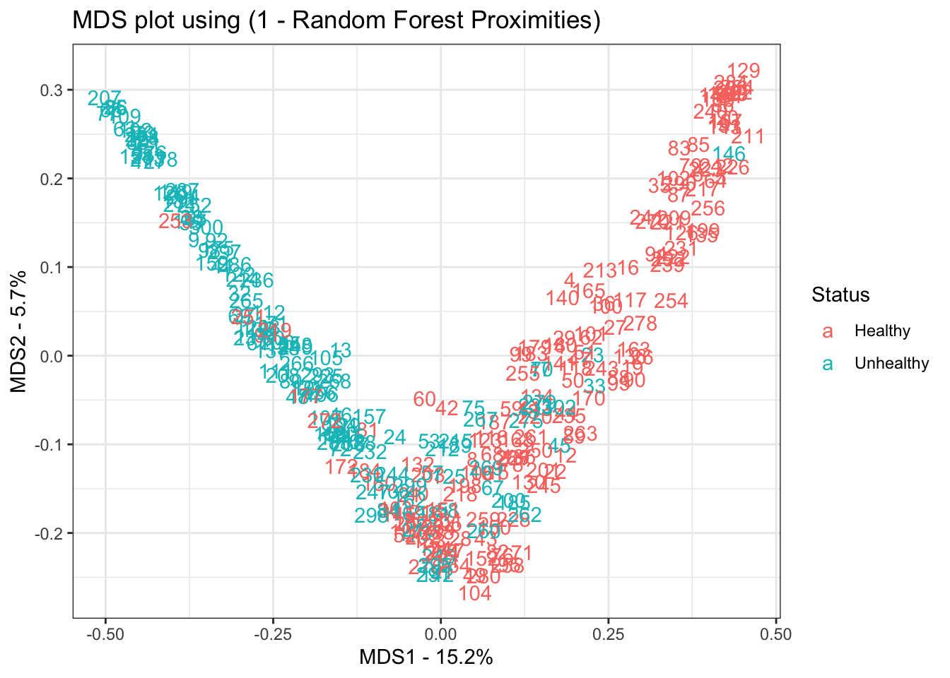

Code

# ggsave(file="random_forest_mds_plot.pdf")